Self-organizing maps

The self-organizing map [1,2] is one of the most prominent artificial neural network models adhering to the unsupervised learning paradigm. The model consists of a number of neural processing elements, i.e. units. Each of the units i is assigned an n-dimensional weight vector m_i. It is important to note that the weight vectors have the same dimensionality as the input patterns.

The training process of self-organizing maps may be described in terms of input pattern presentation and weight vector adaptation. Each training iteration t starts with the random selection of one input pattern x(t). This input pattern is presented to the self-organizing map and each unit determines its activation. Usually, the Euclidean distance between weight vector and input pattern is used to calculate a unit's activation. The unit with the lowest activation is referred to as the winner, c, of the training iteration, i.e.  $m_c(t) = \min_i{\vert\vert x(t)-m_i(t)\vert\vert}$. Finally, the weight vector of the winner as well as the weight vectors of selected units in the vicinity of the winner are adapted. This adaptation is implemented as a gradual reduction of the component-wise difference between input pattern and weight vector, i.e.  $m_i(t+1) = m_i(t) \cdot \alpha(t) \cdot h_{ci}(t) \cdot [x(t)-m_i(t)]$. Geometrically speaking, the weight vectors of the adapted units are moved a bit towards the input pattern. The amount of weight vector movement is guided by a so-called learning rate, $\alpha$, decreasing in time. The number of units that are affected by adaptation is determined by a so-called neighborhood function, h_ci. This number of units also decreases in time. This movement has as a consequence, that the Euclidean distance between those vectors decreases and thus, the weight vectors become more similar to the input pattern. The respective unit is more likely to win at future presentations of this input pattern. The consequence of adapting not only the winner alone but also a number of units in the neighborhood of the winner leads to a spatial clustering of similar input patters in neighboring parts of the self-organizing map. Thus, similarities between input patterns that are present in the n-dimensional input space are mirrored within the two-dimensional output space of the self-organizing map. The training process of the self-organizing map describes a topology preserving mapping from a high-dimensional input space onto a two-dimensional output space where patterns that are similar in terms of the input space are mapped to geographically close locations in the output space.

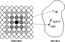
Consider Figure 1 for a graphical representation of self-organizing maps. The map consists of a square arrangement of $7 \times 7$ neural processing elements, i.e. units, shown as circles on the left hand side of the figure. The black circle indicates the unit that was selected as the winner for the presentation of input pattern x(t). The weight vector of the winner, m_c(t), is moved towards the input pattern and thus, m_c(t+1) is nearer to x(t) than was m_c(t). Similar, yet less strong, adaptation is performed with a number of units in the vicinity of the winner. These units are marked as shaded circles in Figure 1. The degree of shading corresponds to the strength of adaptation. Thus, the weight vectors of units shown with a darker shading are moved closer to x than units shown with a lighter shading.

  

Figure: Architecture of a $7 \times 7$ self-organizing map