Music Information Retrieval:
Part 2
Feature Extraction
http://www.ifs.tuwien.ac.at/mir
Alexander Schindler
Research Assistant
Institute of Software Technology and Interactive Systems
Vienna University of Technology
http://www.ifs.tuwien.ac.at/~schindler
This article is a first attempt towards an interactive textbook for the Music Information Retrieval (MIR) part of the Information Retrieval lecture held at the Vienna University of Technology. The content either serves as description of basic music feature extraction as presented in the lecture as well as executable code examples that can be used and extended for the exercises.
Introduction
A typical CD quality mainstream radio track has an average length of three minutes. This means, that the song is digitally described in Pulse-code Modulation (PCM) by allmost 16 million numbers (3 [minutes] x 60 [seconds] x 2 [stereo channels] x 44100 [sampling rate]). This information requires 30MB of memory and a considerable amount of time to process. Processing the small number of 100 tracks, which relates to about 10 audio CDs, would require about 3GB of memory, which is currently about the average size of memory provided in personal computers. Processing 100000 songs would require 3TB of memory, which requires vast ressources (e.g. aquisition, hosting, energy consumption, etc.) and is only suitable for academic or industrial settings.
Consequently, there is a strong desire to reduce the information provided in an audio track an destill it into a smaller set of representative numbers that capture higher level information about the underlying track.
Prerequisites
This article is an IPython Notebook. IPython is a powerful interactive Python shell providing extensive support for data visualization and explorative experimentation. It further provides an interactive browser-based interface with support for code execution, visualization, mathematical expressions and text. This means, that if you have a running IPython Notebook server, you can download and execute this article.
Required Environment
Python
This article demonstrates music feature extraction using the programming language Python, which is a powerful and easy to lean scripting language, providing a rich set of scientific libraries. The examples provided have been coded and tested with Python version 2.7. Since the Python syntax varies considerably between major versions, it is recommended to use the same version.
As explained above this article is an IPython Notebook. Please refere to IPython's Web page for installation instruction.
Python Libraries
The following Python libraries may be not contained in standard Python distributions and may need to be installed additionally:
- Numpy: the fundamental package for scientific computing with Python. It implements a wide range of fast and powerful algebraic functions.
- sklearn: Scikit-Learn is a powerful machine learning package for Python built on numpy and Scientific Python (Scipy).
- Scipy
- scikits.talkbox: Talkbox, a set of python modules for speech/signal processing
Test your Environment
If you have installed all required libraries, the follwing imports should run without errors.
%pylab inline

import warnings
warnings.filterwarnings('ignore')

# numerical processing and scientific libraries
import numpy as np
import scipy

# signal processing
from scipy.io                     import wavfile
from scipy                        import stats, signal
from scipy.fftpack                import fft

from scipy.signal                 import lfilter, hamming
from scipy.fftpack.realtransforms import dct
from scikits.talkbox              import segment_axis
from scikits.talkbox.features     import mfcc

# general purpose
import collections

# plotting
import matplotlib.pyplot as plt
from numpy.lib                    import stride_tricks

from IPython.display              import HTML
from base64                       import b64encode

# Classification and evaluation
from sklearn.preprocessing import StandardScaler
from sklearn import svm
from sklearn.cross_validation import StratifiedKFold, ShuffleSplit, cross_val_score
from sklearn.naive_bayes import GaussianNB
from sklearn.neighbors import KNeighborsClassifier
from sklearn.ensemble import RandomForestClassifier
from sklearn.metrics import classification_report, confusion_matrix

import pandas as pd
Adapt to your local Environment
Some code segments need to be adapted to your local settings (e.g. the paths of the audio files) or you may test the code on different sound files. Code blocks that need to be changed are annotated with the following comment:
### change ###
Music Files
A set of music files will be used to demonstrate different aspects of music feature etraction. The audio tracks used in this article were downloaded from the FreeMusicArchive and are redistributable licensed under the Creative Commons license. To visualize the expressivenmess of music features and their ability to discriminate different types of music, the songs of this article originate from different music genres.
In the code-block below the sound files used in this tutorial will be specified. Please change the paths of the files according your local settings. Because MP3-decoding is not constistently implemented across all platforms, it is required that to manually convert the audio files into wave format as a prerequiste.
# initialize music collection
sound_files = collections.defaultdict(dict)

### change ###
sound_files["Classic"]["path"]         = r"D:\Dropbox\Work\IFS\Lehre\Information Retrieval LVA\IPython\Advent_Chamber_Orchestra_-_04_-_Mozart_-_Eine_Kleine_Nachtmusik_allegro.wav"
sound_files["Classic"]["online_id"]    = 70444

sound_files["Jazz"]["path"]            = r"D:\Dropbox\Work\IFS\Lehre\Information Retrieval LVA\IPython\Michael_Winkle_-_03_-_I_Guess_I_Knew.wav"
sound_files["Jazz"]["online_id"]       = 22974

sound_files["Rock"]["path"]            = r"D:\Dropbox\Work\IFS\Lehre\Information Retrieval LVA\IPython\Room_For_A_Ghost_-_02_-_Burn.wav"
sound_files["Rock"]["online_id"]       = 61491

sound_files["Electronic"]["path"]      = r"D:\Dropbox\Work\IFS\Lehre\Information Retrieval LVA\IPython\Broke_For_Free_-_02_-_Calm_The_Fuck_Down.wav"
sound_files["Electronic"]["online_id"] = 37909

sound_files["Metal"]["path"]           = r"D:\Dropbox\Work\IFS\Lehre\Information Retrieval LVA\IPython\Acrassicauda_-_02_-_Garden_Of_Stones.wav"
sound_files["Metal"]["online_id"]      = 30919

sound_files["Rap"]["path"]             = r"D:\Dropbox\Work\IFS\Lehre\Information Retrieval LVA\IPython\Social_Studies_-_The_Wapner.wav"
sound_files["Rap"]["online_id"]        = 70602
The following code embeds the audio player from the FMA Web page into this notebook. Thus, it is possible to pre-listen the audio samples online.
list_audio_samples(sound_files)
Audio Representations
Basic knowledge of the production process of digital audio is essential to understand how to extract music features and what they express.
Sampling and Quatization
 Audio signals as perceived by our ears have a continuous form. Analog storage media were able to preserve this continuous nature of sound (e.g. vinyl records, music cassttes, etc.). Digital logic circuits on the other hand rely on electronic oscillators that sequentially trigger the unit to process a specific task on a discrete set of data units (e.g. loading data, multiplying registers, etc.). Thus, an audio signal has to be fed in small pieces to the processing unit. The process of reducing a continuous signal to a discrete signal is called sampling. The audio signal is converted into a sequences of discrete numbers that are evenly spaced in time.
As an example one could monitor the temperature in an office by measuring every minute the current degree of Celsius. We fruther simplify this example by accepting only integer values. In this case the continous change of temparature in the office is sampled at a rate of 60 samples per minute. Since Celsius values in offices seldom rise above 128 or drop below -128 degree, it is sufficient to use 8 Bits to store the sampled data. The process of turing continous values (e.g. temperature, sound pressure, etc.) into discrete values is called quantization.
For digitizing audio especially music in CD quality, typically a sampling rate of 44100 Herz at a bit depth of 16 is used. This means, that each second of audio data is represented by 44100 16bit values.
- The time domain
- The frequency domain
- The Fourier Transform
- The Short-Time Fourier Transform
To start the feature extraction process, the audio files have to be opened and loaded. Usually audio files are opened as streams and processed sequentially, but for this tutorial it is more convenient to fully keep them in memory. After the audio data has been loaded two essential data blocks are known: the actual audio data and the rate the source has been sampled with. From this information it is easy to derive the first audio feature: the length of the track. Since the samplerate is defined as number of samples per second, the length is simply calculated by dividing the sample cound by the samplerate.
# load sound files
for genre in sound_files.keys():

    samplerate, wavedata = wavfile.read(sound_files[genre]["path"])

    sound_files[genre]["samplerate"]        = samplerate
    sound_files[genre]["wavedata"]          = wavedata
    sound_files[genre]["number_of_samples"] = wavedata.shape[0]
    sound_files[genre]["song_length"]       = int( sound_files[genre]["number_of_samples"] / samplerate ) # round up
The Time Domain
Time domain analysis is analyzing the data over a time period. Functions such as electronic signals, market behaviors, and biological systems are some of the functions that are analyzed using time domain analysis. For an electronic signal, the time domain analysis is mainly based on the voltage – time plot or the current – time plot. In a time domain analysis, the variable is always measured against time. There are several devices used to analyze data on a time domain basis. The cathode ray oscilloscope (CRO) is the most common device when analyzing electrical signals on a time domain.
Waveform
A waveform is the shape and form of a signal such as a wave moving in a physical medium or an abstract representation.
In many cases the medium in which the wave is being propagated does not permit a direct visual image of the form. In these cases, the term 'waveform' refers to the shape of a graph of the varying quantity against time or distance. An instrument called an oscilloscope can be used to pictorially represent a wave as a repeating image on a screen. By extension, the term 'waveform' also describes the shape of the graph of any varying quantity against time
show_stereo_waveform(sound_files["Classic"]["wavedata"]);

The Frequency Domain
Fourier Transform
Essential part of any audio feature extraction algorithm
Audio waves contain a spectrum of many different frequencies, each with its own amplitude and phase.
Idea is that every complex continuous signal can be explained by decompose a wave into its component frequencies and phases.
- Inverse Fourier Transform Transform back from frequency into time domain
No loss of data when transformation is applied
- Results of the Fourier Transform are
- Phase histogram (rarely used)
- Frequency histogram
- Sets of bins
- Each corresponding to a different range of frequencies
Magnitude Spectrum vs. Power Spectrum
- the power spectrum is the magnitude spectrum squared (calculated for each bin, by summing the square of the imaginary output of the FFT with the square of the real value)
- magnitude spectrum and power spectrum rarely used directly as features (too much raw information)
- many spectral features are derived from either the power spectrum or the magnitude spectrum
Fast Fourier Transform
- efficient algorithm to compute the discrete Fourier transform (DFT)
- divide and conquer algorithm
- \(O(N log N)\) instead of \(O(N2)\)
- \(N\) must be a power of 2
genre = "Rock"

plotstft(sound_files[genre]["wavedata"], sound_files[genre]["samplerate"]);

Audio Pre-processing
Combine separate channels
for genre in sound_files.keys():

    if sound_files[genre]["wavedata"].shape[1] > 1:

        # use combine the channels by calculating their geometric mean
        sound_files[genre]["wavedata"] = np.mean(sound_files[genre]["wavedata"] , axis=1)
Below an example waveform of a mono channel after combining the stereo channels by arithmetic mean:
show_mono_waveform(sound_files["Classic"]["wavedata"])

Audio Features
Time Domain Features
Zero Crossing Rate
Zero-crossing rate is a simple, straightforward and inexpensive feature to examine the similarity between two or more accelerometer sensors. It measures whether two sets of time series measurements exhibit similar patters. It is particularly useful to analyze measurements that are corrupted by noise. For example, a measurement with a high zero-crossing rate, i.e., the number of samples per second that cross the zero reference line, indicates that it is noisy. However, we observe that even for sensors having the same orientation, the calibration error results in a deviation of 40s. Substituting the zero-crossing value by a mean valuecrossing, i.e., by defining a mean threshold that serves as a reference, results in a calibration error with a deviation between 2 and 15/s for individual axes and between 0 and 2/s for the absolute acceleration values of the individual measurements. Cross test of uncorrelated measurements, on the other hand, reveals that the overall calibration error is markedly bigger: between 7 and 50/s for the raw measurements and between 5 and 30/s for the absolute values.
The Zero Crossing Rate (ZCR) is defined by:
\[ zcr = \frac{1}{N-1} \sum_{i=1}^{N-1} | sign|x(i)| - sign|x(i-1)| | \]
where \(N\) is the number of samples of an audio file and the signum function is defined by:
\[ sign|x(i)| = \begin{cases} 1, & \text{ if } x(i) > 0\\ 0, & \text{ if } x(i) = 0\\ -1,&\text{ if } x(i) < 0 \end{cases} \]
average number of times the audio signal crosses the zero amplitude line per time unit. very simple to compute has been applied to speech processing to distinguish voiced sections from noise
also has been applied to MIR tasks such as classifying percussion sounds Genres
def zero_crossing_rate_BruteForce(wavedata):

    zero_crossings = 0

    for i in range(1, number_of_samples):

        if ( wavedata[i - 1] <  0 and wavedata[i] >  0 ) or \
           ( wavedata[i - 1] >  0 and wavedata[i] <  0 ) or \
           ( wavedata[i - 1] != 0 and wavedata[i] == 0):

                zero_crossings += 1

    zero_crossing_rate = zero_crossings / float(number_of_samples - 1)

    return zero_crossing_rate
The following method is numerical more elegant and computationally efficient. It uses the optimized linear algebraic functions of the Numerical Python (numpy) package.
The method further computes the Zero Crossing Rate for a sequence of blocks (also called frames or windows).
def zero_crossing_rate(wavedata, block_length, sample_rate):

    # how many blocks have to be processed?
    num_blocks = int(np.ceil(len(wavedata)/block_length))

    # when do these blocks begin (time in seconds)?
    timestamps = (np.arange(0,num_blocks - 1) * (block_length / float(samplerate)))

    zcr = []

    for i in range(0,num_blocks-1):

        start = i * block_length
        stop  = np.min([(start + block_length - 1), len(wavedata)])

        zc = 0.5 * np.mean(np.abs(np.diff(np.sign(wavedata[start:stop]))))
        zcr.append(zc)

    return np.asarray(zcr), np.asarray(timestamps)
The following charts visualize how the Zero Crossing Rate correlates with the audio signal. The upper chart shows the spectrogram of the track. The lower chart superimposes the Zero Crossing Rate over the waveform of the track. It can be observed that sewuences with increased energy in high frequency reagions have a higher zero crossing rate.
genre = "Rock"

# calculate zero-crossing-rate
zcr, ts = zero_crossing_rate(sound_files[genre]["wavedata"], 2048, sound_files[genre]["samplerate"]);

show_feature_superimposed(genre, zcr, ts);


Use ZCR to compare music
# calculate ZCR for all tracks
for genre in sound_files.keys():

    sound_files[genre]["zcr"], _ = zero_crossing_rate(sound_files[genre]["wavedata"],
                                                      2048,
                                                      sound_files[genre]["samplerate"])
# plot results
plot_compairison(sound_files, "zcr", ["mean"])

plot_compairison(sound_files, "zcr", ["mean", "std"])

Root Mean Square
Root Mean Square is a way of comparing arbitrary waveforms based upon their equivalent energy. RMS voltage is the contant (DC) voltage that would be required to produce the same heat in a resistive load, indicating equivalent ability to do work. You can't use a simple "average voltage": Consider that a sine wave has positive and negative phases that would average to zero, yet it still generates heat regardless of the polarity of the voltage.
The RMS method takes the square of the instantaneous voltage before averaging, then takes the square root of the average. This solves the polarity problem, since the square of a negative value is the same as the square of a positive value. For a sine wave, the RMS value thus computed is the same as the amplitude (zero-to-peak value) divided by the square root of two, or about 0.7071 of the amplitude. For a repetitive waveform like this, an accurate calculation can be done by averaging over a single cycle of the wave (or an integer number of cycles), but for random noise sources the averaging time must be long enough to get a good representation of the characteristics of the source.
For noise or signal bursts, the RMS value is still the effective heating value, but of course it is reduced because the signal is not always present. If you know the RMS value of the continuous signal, the true RMS of the burst will be the continuous RMS times the square root of the fraction of the time the signal is on.
\[r_{rms} = \sqrt{\frac{1}{n} \sum_{i=1}^{n} x_{i}^2}\]
def root_mean_square(wavedata, block_length, sample_rate):

    # how many blocks have to be processed?
    num_blocks = int(np.ceil(len(wavedata)/block_length))

    # when do these blocks begin (time in seconds)?
    timestamps = (np.arange(0,num_blocks - 1) * (block_length / float(samplerate)))

    rms = []

    for i in range(0,num_blocks-1):

        start = i * block_length
        stop  = np.min([(start + block_length - 1), len(wavedata)])

        rms_seg = np.sqrt(np.mean(wavedata[start:stop]**2))
        rms.append(rms_seg)

    return np.asarray(rms), np.asarray(timestamps)
genre = "Rock"

# calculate root-mean-square
rms, ts = root_mean_square(sound_files[genre]["wavedata"], 2048, sound_files[genre]["samplerate"]);

show_feature_superimposed(genre, rms, ts, squared_wf=False);

# calculate Zero Crossing Rate for the collection
for genre in sound_files.keys():

    sound_files[genre]["rms"], _ = root_mean_square(sound_files[genre]["wavedata"],
                                                    2048,
                                                    sound_files[genre]["samplerate"])
# plot results
plot_compairison(sound_files, "rms", ["mean"])

plot_compairison(sound_files, "rms", ["mean", "std"])

Spectral Features
Spectral Shape Features
Spectral Centroid
- center of gravity (balancing point of the spectrum)
- It determines the frequency area around which most of the signal energy concentrates
- gives an indication of how “dark” or “bright” a sound is
The Spectral Centroid \(SC\) is the frequency-weighted sum of the power spectrum (=squared Magnitude spectrum \(M\)) normalized by its unweighted sum:
\[ SC(t) = \frac{\sum_{n=1}^{N}|M(t,n)|^2 * n}{\sum_{n=1}^{N}|M(t,n)|^2} \]
where \(t\) represents the current time frame and \(n\) is the index for one of \(N\) frequency bins calculated by the FFT.
def spectral_centroid(wavedata, window_size, sample_rate):

    magnitude_spectrum = stft(wavedata, window_size)

    timebins, freqbins = np.shape(magnitude_spectrum)

    # when do these blocks begin (time in seconds)?
    timestamps = (np.arange(0,timebins - 1) * (timebins / float(sample_rate)))

    sc = []

    for t in range(timebins-1):

        power_spectrum = np.abs(magnitude_spectrum[t])**2

        sc_t = np.sum(power_spectrum * np.arange(1,freqbins+1)) / np.sum(power_spectrum)

        sc.append(sc_t)


    sc = np.asarray(sc)
    sc = np.nan_to_num(sc)

    return sc, np.asarray(timestamps)
genre = "Metal"

sc, ts = spectral_centroid(sound_files[genre]["wavedata"], 1024, sound_files[genre]["samplerate"])

show_feature_superimposed(genre, sc, ts, squared_wf=False);


# calculate Spectral Centroid for the collection
for genre in sound_files.keys():

    sound_files[genre]["sc"], _ = spectral_centroid(sound_files[genre]["wavedata"],
                                                    1024,
                                                    sound_files[genre]["samplerate"])
plot_compairison(sound_files, "sc", ["mean", "std"])

Spectral Rolloff
- the frequency below which some fraction, k (typically 0.85, 0.9 or 0.95 percentile), of the cumulative spectral power resides
- measure of the skewness of the spectral shape
- indication of how much energy is in the lower frequencies
- It is used to distinguish voiced from unvoiced speech or music
\[ \sum_{n=1}^{SR(t)}|M(t,n)|^2 = n* \sum_{n=1}^{N}|M(t,n)|^2 \]
def spectral_rolloff(wavedata, window_size, sample_rate, k=0.85):

    # convert to frequency domain
    magnitude_spectrum = stft(wavedata, window_size)
    power_spectrum     = np.abs(magnitude_spectrum)**2
    timebins, freqbins = np.shape(magnitude_spectrum)

    # when do these blocks begin (time in seconds)?
    timestamps = (np.arange(0,timebins - 1) * (timebins / float(sample_rate)))

    sr = []

    spectralSum    = np.sum(power_spectrum, axis=1)

    for t in range(timebins-1):

        # find frequency-bin indeces where the cummulative sum of all bins is higher
        # than k-percent of the sum of all bins. Lowest index = Rolloff
        sr_t = np.where(np.cumsum(power_spectrum[t,:]) >= k * spectralSum[t])[0][0]

        sr.append(sr_t)

    sr = np.asarray(sr).astype(float)

    # convert frequency-bin index to frequency in Hz
    sr = (sr / freqbins) * (sample_rate / 2.0)

    return sr, np.asarray(timestamps)
genre = "Classic"

sr, ts = spectral_rolloff(sound_files[genre]["wavedata"],
                           1024,
                           sound_files[genre]["samplerate"],
                           k=0.85)

show_feature_superimposed(genre, sr, ts, squared_wf=False);


# calculate Spectral Rolloff for the collection
for genre in sound_files.keys():

    sound_files[genre]["sr"], _ = spectral_rolloff(sound_files[genre]["wavedata"],
                                                   1024,
                                                   sound_files[genre]["samplerate"],
                                                   k=0.85)
plot_compairison(sound_files, "sr", ["mean", "std"])

Spectral Flux
- squared differences in frequency distribution of two successive time frames
- measures the rate of local change in the spectrum
\[ SF(t) = \frac{\sqrt{\sum_{n=1}^{N}(|M(t,n)| - |M(t-1,n)|)^2} }{N} \]
def spectral_flux(wavedata, window_size, sample_rate):

    # convert to frequency domain
    magnitude_spectrum = stft(wavedata, window_size)
    timebins, freqbins = np.shape(magnitude_spectrum)

    # when do these blocks begin (time in seconds)?
    timestamps = (np.arange(0,timebins - 1) * (timebins / float(sample_rate)))

    sf = np.sqrt(np.sum(np.diff(np.abs(magnitude_spectrum))**2, axis=1)) / freqbins

    return sf[1:], np.asarray(timestamps)
genre = "Classic"

sf, ts = spectral_flux(sound_files[genre]["wavedata"],
                       1024,
                       sound_files[genre]["samplerate"])

show_feature_superimposed(genre, sf, ts);

Spectral Variability
- standard deviation of the bin values of the magnitude spectrum
- provides an indication of how flat the spectrum is and if some frequency regions are much more prominent than others
Strongest Partial
- center frequency of the bin of the magnitude or power spectrum with the greatest strength
- can provide a primitive form of pitch tracking
MPEG7 Features
MPEG-7 is a multimedia content description standard defined by the Moving Picture Expert Group aka MPEG.
- Multimedia Content Description Interface
- ISO/IEC standard by MPEG (Moving Picture Experts Group)
- Providing meta-data for multimedia
- MPEG-1, -2, -4: make content available
- MPEG-7: makes content accessible, retrievable, filterable, manageable (via device / computer).
was Adopted in 2002
- Details:
- ISO/IEC JTC1/SC29/WG11N6828; editor:José M. Martínez Palma de Mallorca, Oct. 2004, MPEG-7 Overview (version 10)
- http://www.chiariglione.org/mpeg/standards/mpeg-7/mpeg-7.htm
- Specifies
- Set of audio descriptors
- a set of Reference Software
Low-level descriptors: * spectral, parametric, and temporal features of a signal
High-level description tools: * specific to a set of applications * general sound recognition and indexing * instrumental timbre * spoken content * audio signature description scheme * melodic description tools to facilitate query-by-humming
MPEG 7 Audio Framework Stack
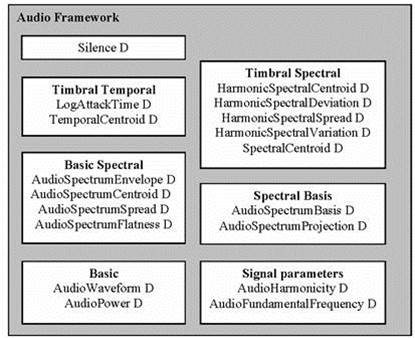
Basic: temporally sampled scalar values for general use. * AudioWaveform Descriptor: waveform envelope for display purposes. * AudioPower Descriptor: temporally-smoothed instantaneous power quick summary of a signal. Applicable to all kinds of signals.
Basic Spectral: single time-frequency analysis of signal * AudioSpectrumEnvelope: Base class. the short-term power spectrum: display, synthesize, general-purpose search * AudioSpectrumCentroid: is the spectrum dominated by high or low frequencies? * AudioSpectrumSpread: the power spectrum centered near the spectral centroid, or spread out over the spectrum? pure-tone and noise-like sounds * AudioSpectrumFlatness: the presence of tonal components
Signal Parameters: periodic or quasi-periodic signals * AudioFundamentalFrequency: “confidence measure”, replacing “pitch-tracking” * AudioHarmonicity: distinction between sounds with a harmonic / inharmonic / non-harmonic spectrum
Timbral Temporal: temporal characteristics of segments of sounds, musical timbre * LogAttackTime * TemporalCentroid: where in time the energy of a signal is focused. Useful when attack times are identical
Timbral Spectral: spectral features in a linear-frequency space * SpectralCentroid: power-weighted average of the frequency of the bins in the linear power spectrum. distinguishing musical instrument timbres. * 4 Ds for harmonic regularly-spaced components of signals: * HarmonicSpectralCentroid * HarmonicSpectralDeviation * HarmonicSpectralSpread * HarmonicSpectralVariation
Spectral Basis: low-dimensional projections of a spectral space to aid compactness and recognition * AudioSpectrumBasis: a series of (time-varying / statistically independent) basis functions derived from the singular value decomposition of a normalized power spectrum. * AudioSpectrumProjection: low-d features of a spectrum after projection upon a reduced rank basis. independent subspaces of a spectra correlate strongly with different sound sources. Provide more salience using less space. With Sound Classification and Indexing Description Tools.
Silence segment: no significant sound * aid further segmentation of the audio stream, or as a hint not to process a segment
Psychoaccoustical Features
Psychoaccoustics
- psychological (subjective) correlations of the physical parameters of acoustics
- Humans are most sensitive to sounds in the 1-5 kHz range
Mel-Frequency Cepstral Coefficients (MFCC)
- used previously in speech recognition
- model human auditory response (Mel scale)
- „cepstrum“ (s-p-e-c reversed): result of taking the Fourier transform (FFT) of the decibel spectrum as if it were a signal
- show rate of change in the different spectrum bands
- Dominant feature in speech recognition, because of ist ability to represent the speech amplitude spectrum in a compact form
- has also prooved to be highly efficient in Music Retrieval
- good timbre feature
- represent the rate of change in the different spectrum bands
The Mel-Scale
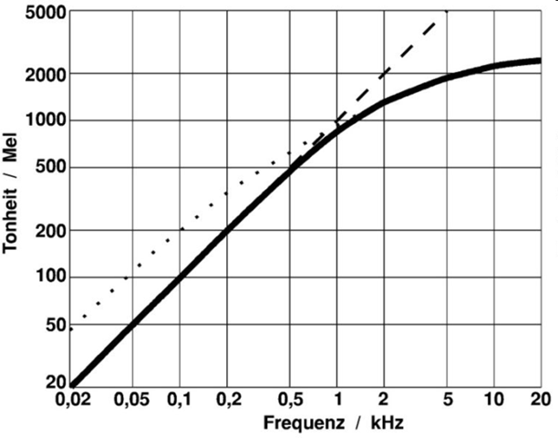
- perceptually motivated scale
- human auditory system does not perceive pitch in linear manner
- Mel comes from the word melody to indicate that the scale is based on pitch comparisons
- maps between actual frequencies and perceived pitch
was obtained empirically by listening experiments
- reference point:
- 1000 Hz tone, 40 dB above listener's threshold = 1000 Mels
- This is the range where humans are most sensitive to variations in sound
- Mapping is approximately
- linear below 1kHz and
- logarhitmic above
MFCC Computiation
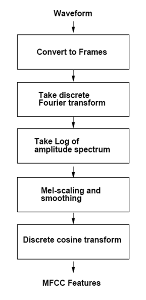
- Pre-processing in time-domain (pre-emphasizing)
- Compute the spectrum amplitude by windowing with a Hamming window
- Filter the signal in the spectral domain with a triangular filter-bank, whose filters are approximatively linearly spaced on the mel scale, and have equal bandwith in the mel scale
- Compute the DCT of the log-spectrum
input_data = sound_files["Classic"]["wavedata"]
Apply pre-filtering
# Pre-emphasis filter.

# Parameters
nwin    = 256
nfft    = 1024
fs      = 16000
nceps   = 13

# Pre-emphasis factor (to take into account the -6dB/octave
# rolloff of the radiation at the lips level)
prefac  = 0.97

# MFCC parameters: taken from auditory toolbox
over    = nwin - 160

filtered_data = lfilter([1., -prefac], 1, input_data)
Compute the spectrum amplitude by windowing with a Hamming window
windows     = hamming(256, sym=0)
framed_data = segment_axis(filtered_data, nwin, over) * windows

# Compute the spectrum magnitude
magnitude_spectrum = np.abs(fft(framed_data, nfft, axis=-1))
Filter the signal in the spectral domain with a triangular filter-bank, whose filters are approximatively linearly spaced on the mel scale, and have equal bandwith in the mel scale
# Compute triangular filterbank for MFCC computation.

lowfreq  = 133.33
linsc    = 200/3.
logsc    = 1.0711703
fs = 44100

nlinfilt = 13
nlogfilt = 27

# Total number of filters
nfilt    = nlinfilt + nlogfilt

#------------------------
# Compute the filter bank
#------------------------
# Compute start/middle/end points of the triangular filters in spectral
# domain
freqs            = np.zeros(nfilt+2)
freqs[:nlinfilt] = lowfreq + np.arange(nlinfilt) * linsc
freqs[nlinfilt:] = freqs[nlinfilt-1] * logsc ** np.arange(1, nlogfilt + 3)
heights          = 2./(freqs[2:] - freqs[0:-2])

# Compute filterbank coeff (in fft domain, in bins)
filterbank  = np.zeros((nfilt, nfft))

# FFT bins (in Hz)
nfreqs = np.arange(nfft) / (1. * nfft) * fs

for i in range(nfilt):

    low = freqs[i]
    cen = freqs[i+1]
    hi  = freqs[i+2]

    lid    = np.arange(np.floor(low * nfft / fs) + 1,
                       np.floor(cen * nfft / fs) + 1, dtype=np.int)

    rid    = np.arange(np.floor(cen * nfft / fs) + 1,
                       np.floor(hi * nfft / fs)  + 1, dtype=np.int)

    lslope = heights[i] / (cen - low)
    rslope = heights[i] / (hi - cen)

    filterbank[i][lid] = lslope * (nfreqs[lid] - low)
    filterbank[i][rid] = rslope * (hi - nfreqs[rid])
Filter the spectrum through the triangle filterbank
# apply filter
mspec = np.log10(np.dot(magnitude_spectrum, filterbank.T))
fig, ax = plt.subplots(2, 1, sharey=True, figsize=(PLOT_WIDTH, 5.5))
cax = ax[0].imshow(np.transpose(magnitude_spectrum), origin="lower", aspect="auto",  interpolation="nearest")
cax = ax[1].imshow(np.transpose(mspec), origin="lower", aspect="auto",  interpolation="nearest")
plt.show()

Compute the MFCC by computing the DCT of the log-spectrum
# Use the DCT to 'compress' the coefficients (spectrum -> cepstrum domain)
MFCCs = dct(mspec, type=2, norm='ortho', axis=-1)[:, :nceps]
MFCCs, mspec, spec = mfcc(sound_files["Rock"]["wavedata"])

fig, ax = plt.subplots(1, 1, sharey=True, figsize=(PLOT_WIDTH, 3.5))
cax = ax.imshow(np.transpose(MFCCs), origin="lower", aspect="auto",  interpolation="nearest")
plt.show()

Rhythm Patterns
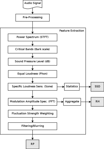 Rhythm Patterns (also called Fluctuation Patterns) describe modulation amplitudes for a range of modulation frequencies on "critical bands" of the human auditory range, i.e. fluctuations (or rhythm) on a number of frequency bands. The feature extraction process for the Rhythm Patterns is composed of two stages:
First, the specific loudness sensation in different frequency bands is computed, by using a Short Time FFT, grouping the resulting frequency bands to psycho-acoustically motivated critical-bands, applying spreading functions to account for masking effects and successive transformation into the decibel, Phon and Sone scales. This results in a power spectrum that reflects human loudness sensation (Sonogram).
In the second step, the spectrum is transformed into a time-invariant representation based on the modulation frequency, which is achieved by applying another discrete Fourier transform, resulting in amplitude modulations of the loudness in individual critical bands. These amplitude modulations have different effects on human hearing sensation depending on their frequency, the most significant of which, referred to as fluctuation strength, is most intense at 4 Hz and decreasing towards 15 Hz. From that data, reoccurring patterns in the individual critical bands, resembling rhythm, are extracted, which – after applying Gaussian smoothing to diminish small variations – result in a time-invariant, comparable representation of the rhythmic patterns in the individual critical bands.
Options
Read Wave File
Read wave file from disk. Only wave input is currently supported. It is intended to leave it that way - the calling application has to take care of the decoding and has to provide pcm data.
data = sound_files["Rock"]["wavedata"]
fs   = sound_files["Rock"]["samplerate"]
# Parameters
skip_leadin_fadeout = 1
step_width          = 3

segment_size        = 2**18
fft_window_size     = 1024   # for 44100 Hz

# Pre-calculate required values

duration  =  data.shape[0]/fs

# calculate frequency values on y-axis (for bark scale calculation)
freq_axis = float(fs)/fft_window_size * np.arange(0,(fft_window_size/2) + 1)

# modulation frequency x-axis (after 2nd fft)
mod_freq_res  = 1 / (float(segment_size) / fs) # resolution of modulation
                                               # frequency axis (0.17 Hz)
mod_freq_axis = mod_freq_res * np.arange(257)  # modulation frequencies along
                                               # x-axis from index 1 to 257)

fluct_curve   = 1 / (mod_freq_axis/4 + 4/mod_freq_axis)
find position of wave segment
skip_seg = skip_leadin_fadeout

seg_pos = np.array([1, segment_size])

if ((skip_leadin_fadeout > 0) or (step_width > 1)):

    if (duration < 45):

        # if file is too small, don't skip leadin/fadeout and set step_width to 1
        step_width = 1
        skip_seg   = 0

    else:
        seg_pos = seg_pos + segment_size * skip_seg; # advance by number of skip_seg segments (i.e. skip lead_in)

# values verified
extract wave segment that will be processed
wavsegment = data[seg_pos[0]-1:seg_pos[1]]
adjust hearing threshold
wavsegment = 0.0875 * wavsegment * (2**15)

plot(wavsegment);

Convert to frequency domain
# [S1] spectrogram: real FFT with hanning window and 50 % overlap

# number of iterations with 50% overlap
n_iter = wavsegment.shape[0] / fft_window_size * 2 - 1
w      = np.hanning(fft_window_size)

spectrogr = np.zeros((fft_window_size/2 + 1, n_iter))

idx = np.arange(fft_window_size)

# stepping through the wave segment,
# building spectrum for each window
for i in range(n_iter):

    spectrogr[:,i] = periodogram(x=wavsegment[idx], win=w)
    idx = idx + fft_window_size/2
Pxx = spectrogr
pylab.figure()
pylab.imshow((spectrogr), origin='lower', aspect='auto',interpolation='nearest')
pylab.xlabel('Time')
pylab.ylabel('Frequency')
pylab.show()

Map to Bark Scale
Bark Scale
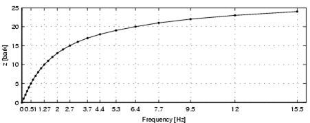
- psychoacoustical scale (related to Mel scale)
- proposed by Eberhard Zwicker in 1961
- named after Heinrich Barkhausen who proposed the first subjective measurements of loudness
- 24 „critical bands“ of hearing (non linear)
- a frequency scale on which equal distances correspond with perceptually equal distances
- Associated to mel scale: 1 Bark corresponds to 100 mel
Prepare Bark-filterbanks
# border definitions of the 24 critical bands of hearing
bark = [100,   200,  300,  400,  510,  630,   770,   920,
        1080, 1270, 1480, 1720, 2000, 2320,  2700,  3150,
        3700, 4400, 5300, 6400, 7700, 9500, 12000, 15500]

eq_loudness = np.array(
    [[ 55,   40,  32,  24,  19,  14, 10,  6,  4,  3,  2,
        2,    0,  -2,  -5,  -4,   0,  5, 10, 14, 25, 35],
     [ 66,   52,  43,  37,  32,  27, 23, 21, 20, 20, 20,
       20,   19,  16,  13,  13,  18, 22, 25, 30, 40, 50],
     [ 76,   64,  57,  51,  47,  43, 41, 41, 40, 40, 40,
     39.5, 38,  35,  33,  33,  35, 41, 46, 50, 60, 70],
     [ 89,   79,  74,  70,  66,  63, 61, 60, 60, 60, 60,
       59,   56,  53,  52,  53,  56, 61, 65, 70, 80, 90],
     [103,   96,  92,  88,  85,  83, 81, 80, 80, 80, 80,
       79,   76,  72,  70,  70,  75, 79, 83, 87, 95,105],
     [118,  110, 107, 105, 103, 102,101,100,100,100,100,
       99,   97,  94,  90,  90,  95,100,103,105,108,115]])

loudn_freq = np.array(
    [31.62,   50,  70.7,   100, 141.4,   200, 316.2,  500,
     707.1, 1000,  1414,  1682,  2000,  2515,  3162, 3976,
     5000,  7071, 10000, 11890, 14140, 15500])

# calculate bark-filterbank
loudn_bark = np.zeros((eq_loudness.shape[0], len(bark)))

i = 0
j = 0

for bsi in bark:

    while j < len(loudn_freq) and bsi > loudn_freq[j]:
        j += 1

    j -= 1

    if np.where(loudn_freq == bsi)[0].size != 0: # loudness value for this frequency already exists
        loudn_bark[:,i] = eq_loudness[:,np.where(loudn_freq == bsi)][:,0,0]
    else:
        w1 = 1 / np.abs(loudn_freq[j] - bsi)
        w2 = 1 / np.abs(loudn_freq[j + 1] - bsi)
        loudn_bark[:,i] = (eq_loudness[:,j]*w1 + eq_loudness[:,j+1]*w2) / (w1 + w2)

    i += 1
Apply Bark-Filter
matrix = np.zeros((len(bark),Pxx.shape[1]))

barks = bark[:]
barks.insert(0,0)

for i in range(len(barks)-1):

    matrix[i] = np.sum(Pxx[((freq_axis >= barks[i]) & (freq_axis < barks[i+1]))], axis=0)
pylab.figure()
pylab.imshow(matrix, origin='lower', aspect='auto',interpolation='nearest')
pylab.xlabel('Time')
pylab.ylabel('Frequency')
pylab.show()

Spectral Masking
- Occlusion of a quiet sound by a louder sound when both sounds are present simultaneously and have similar frequencies
- Simultaneous masking: two sounds active simultaneously
- Post-masking: a sound closely following it (100-200 ms)
- Pre-masking: a sound preceding it (usually neglected, only measured during about 20ms)
- Spreading function defining the influence of the \(j\)-th critical band on the \(i\)-th
For Example: * A quiet sound is masked by a loud sound that has the same frequency * if both are played simultaneously * if the are played very close to each other
# SPREADING FUNCTION FOR SPECTRAL MASKING
# CONST_spread contains matrix of spectral frequency masking factors
n_bark_bands = len(bark)

CONST_spread = np.zeros((n_bark_bands,n_bark_bands))

for i in range(n_bark_bands):
    CONST_spread[i,:] = 10**((15.81+7.5*((i-np.arange(n_bark_bands))+0.474)-17.5*(1+((i-np.arange(n_bark_bands))+0.474)**2)**0.5)/10)

spread = CONST_spread[0:matrix.shape[0],:]
matrix = np.dot(spread, matrix)
pylab.figure()
pylab.imshow(matrix, origin='lower', aspect='auto',interpolation='nearest')
pylab.xlabel('Time')
pylab.ylabel('Frequency')
pylab.show()

Map to Decibel Scale
Transform the energy values on the critical bands into decibel scale
matrix[np.where(matrix < 1)] = 1

matrix = 10 * np.log10(matrix)
pylab.figure()
pylab.imshow(matrix, origin='lower', aspect='auto',interpolation='nearest')
pylab.xlabel('Time')
pylab.ylabel('Frequency')
pylab.show()

Transform to Phon Scale
Equal loudness curves (Phon)
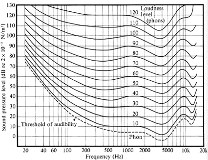
- Represents the relationship between the sound pressure level in decibel and the perceived hearing sensation.
- This relationship is not linear and depends on the frequency of the tone
- Centered around 1khz
- equal loudness contours for 3, 20, 40, 60, 80, 100 phon
- To perceive a 40Hz tone with the same sensation sf loudness, 5 times more sound presure is required.
Compute specific loudness sensation per critical band
# phon-mappings
phon = [3, 20, 40, 60, 80, 100, 101]


# number of bark bands, matrix length in time dim
n_bands = matrix.shape[0]
t       = matrix.shape[1]

# DB-TO-PHON BARK-SCALE-LIMIT TABLE
# introducing 1 level more with level(1) being infinite
# to avoid (levels - 1) producing errors like division by 0


table_dim = n_bands;
cbv       = np.concatenate((np.tile(np.inf,(table_dim,1)),
                            loudn_bark[:,0:n_bands].transpose()),1)

phons     = phon[:]
phons.insert(0,0)
phons     = np.asarray(phons)

# init lowest level = 2
levels = np.tile(2,(n_bands,t))

for lev in range(1,6):
    db_thislev = np.tile(np.asarray([cbv[:,lev]]).transpose(),(1,t))
    levels[np.where(matrix > db_thislev)] = lev + 2

# the matrix 'levels' stores the correct Phon level for each datapoint
cbv_ind_hi = np.ravel_multi_index(dims=(table_dim,7), multi_index=np.array([np.tile(np.array([range(0,table_dim)]).transpose(),(1,t)), levels-1]), order='F')
cbv_ind_lo = np.ravel_multi_index(dims=(table_dim,7), multi_index=np.array([np.tile(np.array([range(0,table_dim)]).transpose(),(1,t)), levels-2]), order='F')

# interpolation factor % OPT: pre-calc diff
ifac = (matrix[:,0:t] - cbv.transpose().ravel()[cbv_ind_lo]) / (cbv.transpose().ravel()[cbv_ind_hi] - cbv.transpose().ravel()[cbv_ind_lo])

ifac[np.where(levels==2)] = 1 # keeps the upper phon value;
ifac[np.where(levels==8)] = 1 # keeps the upper phon value;

matrix[:,0:t] = phons.transpose().ravel()[levels - 2] + (ifac * (phons.transpose().ravel()[levels - 1] - phons.transpose().ravel()[levels - 2])) # OPT: pre-calc diff
pylab.figure()
pylab.imshow(matrix, origin='lower', aspect='auto',interpolation='nearest')
pylab.xlabel('Time')
pylab.ylabel('Frequency')
pylab.show()

Transform to Sone Scale
Sone Transformation
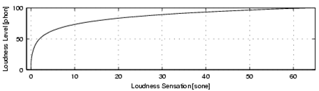
- Perceived loudness measured in Phon does not increase linearly
- Transformation into Sone
- Up to 40 phon slow increase in perceived loudness, then drastic increase
- Higher sensibility for certain loudness differences
Sone 1 2 4 8 16 32 64
Phon 40 50 60 70 80 90 100
idx     = np.where(matrix >= 40)
not_idx = np.where(matrix < 40)

matrix[idx]     =  2**((matrix[idx]-40)/10)
matrix[not_idx] =  (matrix[not_idx]/40)**2.642

# values verified
pylab.figure()
pylab.imshow(matrix, origin='lower', aspect='auto',interpolation='nearest')
pylab.xlabel('Time')
pylab.ylabel('Frequency')
pylab.show()

Statistical Spectrum Descriptors
The Sonogram is calculated as in the first part of the Rhythm Patterns calculation. According to the occurrence of beats or other rhythmic variation of energy on a specific critical band, statistical measures are able to describe the audio content. Our goal is to describe the rhythmic content of a piece of audio by computing the following statistical moments on the Sonogram values of each of the critical bands: mean, median, variance, skewness, kurtosis, min- and max-value
def calc_statistical_features(mat):

    result = np.zeros((mat.shape[0],7))

    result[:,0] = np.mean(mat, axis=1)
    result[:,1] = np.var(mat, axis=1)
    result[:,2] = scipy.stats.skew(mat, axis=1)
    result[:,3] = scipy.stats.kurtosis(mat, axis=1)
    result[:,4] = np.median(mat, axis=1)
    result[:,5] = np.min(mat, axis=1)
    result[:,6] = np.max(mat, axis=1)

    result = np.nan_to_num(result)

    return result
ssd = calc_statistical_features(matrix)

ssd.shape
Rhythm Patterns
Calculate fluctuation patterns from scaled spectrum
# calculate fft window-size
fft_size = 2**(nextpow2(matrix.shape[1]))

rhythm_patterns = np.zeros((matrix.shape[0], fft_size), dtype=complex128)

# calculate fourier transform for each bark scale
for b in range(0,matrix.shape[0]):

    rhythm_patterns[b,:] = fft(matrix[b,:], fft_size)

# normalize results
rhythm_patterns = rhythm_patterns / 256

# take first 60 values of fft result including DC component
feature_part_xaxis_rp = range(0,60)

rp = np.abs(rhythm_patterns[:,feature_part_xaxis_rp])
pylab.figure()
pylab.imshow(rp, origin='lower', aspect='auto',interpolation='nearest')
pylab.xlabel('Time')
pylab.ylabel('Frequency')
pylab.show()

Rhythm Histograms
The Rhythm Histogram features we use are a descriptor for general rhythmics in an audio document. Contrary to the Rhythm Patterns and the Statistical Spectrum Descriptor, information is not stored per critical band. Rather, the magnitudes of each modulation frequency bin of all critical bands are summed up, to form a histogram of "rhythmic energy" per modulation frequency. The histogram contains 60 bins which reflect modulation frequency between 0 and 10 Hz. For a given piece of audio, the Rhythm Histogram feature set is calculated by taking the median of the histograms of every 6 second segment processed.
rh = np.sum(np.abs(rhythm_patterns[:,feature_part_xaxis_rp]),axis=0)
fig, ax = plt.subplots()
ax.bar(range(rh.shape[0]),rh)
plt.show();

Modulation Variance Descriptors
This descriptor measures variations over the critical frequency bands for a specific modulation frequency (derived from a rhythm pattern).
Considering a rhythm pattern, i.e. a matrix representing the amplitudes of 60 modulation frequencies on 24 critical bands, an MVD vector is derived by computing statistical measures (mean, median, variance, skewness, kurtosis, min and max) for each modulation frequency over the 24 bands. A vector is computed for each of the 60 modulation frequencies. Then, an MVD descriptor for an audio file is computed by the mean of multiple MVDs from the audio file's segments, leading to a 420-dimensional vector.
mvd = calc_statistical_features(rp.transpose())
Music Similarity Retrieval
Load extracted features from prepared files
feature_files = [["zcr", r"D:\MIR\Data\AudioVideo\Features\Audio\MV-VIS\mv-vis.marsyas.noFilename.zcr.npz"],
                 ["sc",  r"D:\MIR\Data\AudioVideo\Features\Audio\MV-VIS\mv-vis.marsyas.noFilename.SpectralCentroid.npz"],
                 ["sf",  r"D:\MIR\Data\AudioVideo\Features\Audio\MV-VIS\mv-vis.marsyas.noFilename.SpectralFlus.npz"],
                 ["sr",  r"D:\MIR\Data\AudioVideo\Features\Audio\MV-VIS\mv-vis.marsyas.noFilename.SpectralRolloff.npz"],
                 ["mfcc",r"D:\MIR\Data\AudioVideo\Features\Audio\MV-VIS\mv-vis.marsyas.noFilename.MFCC.npz"],
                 ["ssd", r"D:\MIR\Data\AudioVideo\Features\Audio\MV-VIS\mv-vis.ssd.noFilename.npz"],
                 ["rp",  r"D:\MIR\Data\AudioVideo\Features\Audio\MV-VIS\mv-vis.rp.npz"],
                 ["rh",  r"D:\MIR\Data\AudioVideo\Features\Audio\MV-VIS\mv-vis.rh.npz"]]

features = {}

for f_name, ff in feature_files:

    dat = np.load(ff)

    features[f_name] = {}

    features[f_name]["labels"]        = dat["labels"]
    features[f_name]["filenames"]     = dat["filenames_mar"]
    features[f_name]["data"]          = dat["data"]

    dat.close()

features["ssd_rp"] = {}
features["ssd_rp"]["data"]          = np.concatenate([features["ssd"]["data"],
                                                      features["rp"]["data"]],axis=1)


for f_name in features.keys():
    features[f_name]["filenames"] = features["rp"]["filenames"]
    features[f_name]["labels"]    = features["zcr"]["labels"]

map_labels_to_numbers(features)
Feature space pre-processing
Normalization * to reduce the influence of outliers * Standard Score - Zero Mean and Unit Variance \[ z = {x- \mu \over \sigma} \]
for f_name in features.keys():
    features[f_name]["data"] = ((features[f_name]["data"] -
                                 np.mean(features[f_name]["data"],axis=0))
                                / np.std(features[f_name]["data"],axis=0))
Nearest Neighbor Search
- Music Similarity based on vector similarity
Requires a similarity metric or measure:
- Manhattan Distance (L1) \[ d(p,q) = \sum_{i=1}^n |q_i-p_i| \]
- Euclidean Distance (L2) \[ d(p,q) = \sqrt{\sum_{i=1}^n (q_i-p_i)^2} \]
- for distance measures vectors with smaller distances are more similar
rank results by ascending distance or descending similarity
feature_set  = "ssd"

cur_instance = 455 # Metal
#cur_instance = 219 # Dance
#cur_instance = 319 # Latin

print "\nsearch similar songs for:\n"
print features[feature_set]["filenames"][cur_instance]
print "=========================\n"

# calculate Manhattan Distance
distances_l1 = ((np.abs(features[feature_set]["data"] -
                     features[feature_set]["data"][cur_instance,:]))
             ).sum(axis=1)

# calculate Euclidean Distance
distances_l2 = np.sqrt((((features[feature_set]["data"] -
                     features[feature_set]["data"][cur_instance,:]))**2
             ).sum(axis=1))

# sort dataset by similarity
sorted_dist_idx = np.argsort(distances_l1)

# display results
for i in [0,1,2,3,4,5,6,7,8,9,10,20,50,100,200,500]:

    print "{0:3d}: {1}".format(i, features[feature_set]["filenames"][sorted_dist_idx[i]])
Music Classification
Genre Classification
feature_set = "mfcc"
Partition the data set. Create a subset that can be used to train the classifier and another to evaluate it.
sp = ShuffleSplit(features[feature_set]["num_labels"].shape[0], # number of tracks
                  n_iter=1,
                  test_size=.25)                                # size of test split

train_split, test_split = zip(*sp)

test_split
Create the classifier. In this example we use a K-Nearest Neighbor classifier with k=1.
classifier = KNeighborsClassifier(n_neighbors=1)
Train the classifier on the feature values with the previously created partition.
classifier.fit(features[feature_set]["data"][train_split],
               features[feature_set]["num_labels"][train_split])
Predict genre label for all tracks of the test set based on the feature vector
for idx in sorted(test_split[0]):

    num_label = classifier.predict(features[feature_set]["data"][idx,:])[0]

    print "{0:10s} => {1}".format(features[feature_set]["labels"][idx],
                    features[feature_set]["num_to_label"][num_label])
Evaluate Classification Experiments
Classification Metrics
feature_set = "mfcc"

classifier.fit(features[feature_set]["data"][train_split],
               features[feature_set]["num_labels"][train_split])

predictions = classifier.predict(features[feature_set]["data"][test_split])

print(classification_report(features[feature_set]["num_labels"][test_split],
                            predictions,
                            target_names=features[feature_set]["num_to_label"]))
Confusion Matrix
cm = confusion_matrix(features[feature_set]["num_labels"][test_split],
                      predictions)

print cm

fig, ax = plt.subplots()

x = range(len(features[feature_set]["num_to_label"]))
plt.xticks(x,  features[feature_set]["num_to_label"])
plt.yticks(x,  features[feature_set]["num_to_label"])
locs, labels = plt.xticks()
plt.setp(labels, rotation=90)
plt.imshow(cm, aspect='auto',interpolation='nearest', cmap='gray');

Cross Validation
crossvalidation = StratifiedKFold(features[feature_set]["num_labels"], n_folds=10)

scores = cross_val_score(classifier,
                         features[feature_set]["data"],
                         features[feature_set]["num_labels"],
                         scoring='accuracy',
                         cv=crossvalidation)

print("Accuracy: %0.2f (+/- %0.2f)" % (scores.mean(), scores.std() * 2))
Compare performance of all features
Run classification experiments
# classifiers used for evaluation
classifiers = {}

classifiers["GNB"]        = GaussianNB()
classifiers["svm_linear"] = svm.SVC(kernel='linear', C=0.3)
classifiers["knn"]        = KNeighborsClassifier(n_neighbors=1)
classifiers["RF"]         = RandomForestClassifier(n_estimators=10,
                                                   criterion='gini',
                                                   n_jobs=-1)

crossvalidation = StratifiedKFold(features[feature_set]["num_labels"], n_folds=4)

# run k-fold cross-validation
for train, test in crossvalidation:

    for f_name in features.keys():

        features[f_name]["results"] = {}

        # evaluate performance of feature set on each classifier
        for c_name, classifier in classifiers.items():

            if c_name not in features[f_name]["results"]:
                features[f_name]["results"][c_name] = []

            classifier.fit(features[f_name]["data"][train],
                           features[f_name]["num_labels"][train])

            result = classifier.score(features[f_name]["data"][test],
                                      features[f_name]["num_labels"][test])

            features[f_name]["results"][c_name].append( result )
Display summary of results measured in mean classification accuracy.
index_labels = []
results_data = []

for df_name in sorted(features.keys()):

    index_labels.append(df_name)

    row_dat = []
    for cf in classifiers.keys():

        vals = features[df_name]["results"][cf]
        row_dat.append(np.mean(vals) * 100)

    results_data.append(row_dat)

warnings.filterwarnings("ignore", category=DeprecationWarning, module="pandas", lineno=570)
pd.DataFrame(np.asarray(results_data), index=index_labels, columns=classifiers.keys())
References
Thomas Lidy, Andreas Rauber. Evaluation of Feature Extractors and Psycho-acoustic Transformations for Music Genre Classification. Proceedings of the Sixth International Conference on Music Information Retrieval (ISMIR 2005), pp. 34-41, London, UK, September 11-15, 2005. PDF
A. Rauber, E. Pampalk, D. Merkl. The SOM-enhanced JukeBox: Organization and Visualization of Music Collections based on Perceptual Models. In: Journal of New Music Research (JNMR), 32(2):193-210, Swets and Zeitlinger, June 2003. Abstract
A. Rauber, and M. Frühwirth. Automatically Analyzing and Organizing Music Archives. In: Proceedings of the 5. European Conference on Research and Advanced Technology for Digital Libraries (ECDL 2001), Sept. 4-8 2001, Darmstadt, Germany, Springer Lecture Notes in Computer Science, Springer, 2001. PDF
.. [1] S.B. Davis and P. Mermelstein, "Comparison of parametric representations for monosyllabic word recognition in continuously spoken sentences", IEEE Trans. Acoustics. Speech, Signal Proc. ASSP-28 (4): 357-366, August 1980."""
Download
Software for the extraction of Rhythm Patterns, Statistical Spectrum Descriptors, Rhythm Histograms, Modulation Frequency Variance Descriptor, Temporal Statistical Spectrum Descriptors and Temporal Rhythm Histograms is available from the download section.
Utility Functions
ABBRIVATIONS = {}

# features
ABBRIVATIONS["zcr"] = "Zero Crossing Rate"
ABBRIVATIONS["rms"] = "Root Mean Square"
ABBRIVATIONS["sc"]  = "Spectral Centroid"
ABBRIVATIONS["sf"]  = "Spectral Flux"
ABBRIVATIONS["sr"]  = "Spectral Rolloff"

# aggregations
ABBRIVATIONS["var"] = "Variance"
ABBRIVATIONS["std"] = "Standard Deviation"
ABBRIVATIONS["mean"] = "Average"

PLOT_WIDTH  = 15
PLOT_HEIGHT = 3.5


def show_mono_waveform(samples):

	fig = plt.figure(num=None, figsize=(PLOT_WIDTH, PLOT_HEIGHT), dpi=72, facecolor='w', edgecolor='k')

	channel_1 = fig.add_subplot(111)
	channel_1.set_ylabel('Channel 1')
	#channel_1.set_xlim(0,song_length) # todo
	channel_1.set_ylim(-32768,32768)

	channel_1.plot(samples)

	plt.show();
	plt.clf();

def show_stereo_waveform(samples):

	fig = plt.figure(num=None, figsize=(PLOT_WIDTH, 5), dpi=72, facecolor='w', edgecolor='k')

	channel_1 = fig.add_subplot(211)
	channel_1.set_ylabel('Channel 1')
	#channel_1.set_xlim(0,song_length) # todo
	channel_1.set_ylim(-32768,32768)
	channel_1.plot(samples[:,0])

	channel_2 = fig.add_subplot(212)
	channel_2.set_ylabel('Channel 2')
	channel_2.set_xlabel('Time (s)')
	channel_2.set_ylim(-32768,32768)
	#channel_2.set_xlim(0,song_length) # todo
	channel_2.plot(samples[:,1])

	plt.show();
	plt.clf();


""" short time fourier transform of audio signal """
def stft(sig, frameSize, overlapFac=0.5, window=np.hanning):
    win = window(frameSize)
    hopSize = int(frameSize - np.floor(overlapFac * frameSize))

    # zeros at beginning (thus center of 1st window should be for sample nr. 0)
    samples = np.append(np.zeros(np.floor(frameSize/2.0)), sig)
    # cols for windowing
    cols = np.ceil( (len(samples) - frameSize) / float(hopSize)) + 1
    # zeros at end (thus samples can be fully covered by frames)
    samples = np.append(samples, np.zeros(frameSize))

    frames = stride_tricks.as_strided(samples, shape=(cols, frameSize), strides=(samples.strides[0]*hopSize, samples.strides[0])).copy()
    frames *= win

    return np.fft.rfft(frames)

""" scale frequency axis logarithmically """
def logscale_spec(spec, sr=44100, factor=20.):
    timebins, freqbins = np.shape(spec)

    scale = np.linspace(0, 1, freqbins) ** factor
    scale *= (freqbins-1)/max(scale)
    scale = np.unique(np.round(scale))

    # create spectrogram with new freq bins
    newspec = np.complex128(np.zeros([timebins, len(scale)]))
    for i in range(0, len(scale)):
        if i == len(scale)-1:
            newspec[:,i] = np.sum(spec[:,scale[i]:], axis=1)
        else:
            newspec[:,i] = np.sum(spec[:,scale[i]:scale[i+1]], axis=1)

    # list center freq of bins
    allfreqs = np.abs(np.fft.fftfreq(freqbins*2, 1./sr)[:freqbins+1])
    freqs = []
    for i in range(0, len(scale)):
        if i == len(scale)-1:
            freqs += [np.mean(allfreqs[scale[i]:])]
        else:
            freqs += [np.mean(allfreqs[scale[i]:scale[i+1]])]

    return newspec, freqs

""" plot spectrogram"""
def plotstft(samples, samplerate, binsize=2**10, plotpath=None, colormap="jet", ax=None, fig=None):

    s = stft(samples, binsize)

    sshow, freq = logscale_spec(s, factor=1.0, sr=samplerate)
    ims = 20.*np.log10(np.abs(sshow)/10e-6) # amplitude to decibel

    timebins, freqbins = np.shape(ims)

    if ax is None:
        fig, ax = plt.subplots(1, 1, sharey=True, figsize=(PLOT_WIDTH, 3.5))

    #ax.figure(figsize=(15, 7.5))
    cax = ax.imshow(np.transpose(ims), origin="lower", aspect="auto", cmap=colormap, interpolation="none")
    #cbar = fig.colorbar(cax, ticks=[-1, 0, 1], cax=ax)
    #ax.set_colorbar()

    ax.set_xlabel("time (s)")
    ax.set_ylabel("frequency (hz)")
    ax.set_xlim([0, timebins-1])
    ax.set_ylim([0, freqbins])

    xlocs = np.float32(np.linspace(0, timebins-1, 5))
    ax.set_xticks(xlocs, ["%.02f" % l for l in ((xlocs*len(samples)/timebins)+(0.5*binsize))/samplerate])
    ylocs = np.int16(np.round(np.linspace(0, freqbins-1, 10)))
    ax.set_yticks(ylocs, ["%.02f" % freq[i] for i in ylocs])

    if plotpath:
        plt.savefig(plotpath, bbox_inches="tight")
    else:
        plt.show()

    #plt.clf();
    b = ["%.02f" % l for l in ((xlocs*len(samples)/timebins)+(0.5*binsize))/samplerate]
    return xlocs, b, timebins


def list_audio_samples(sound_files):

	src = ""

	for genre in sound_files.keys():

		src += "<b>" + genre + "</b><br><br>"
		src += "<object width='600' height='90'><param name='movie' value='http://freemusicarchive.org/swf/trackplayer.swf'/><param name='flashvars' value='track=http://freemusicarchive.org/services/playlists/embed/track/{0}.xml'/><param name='allowscriptaccess' value='sameDomain'/><embed type='application/x-shockwave-flash' src='http://freemusicarchive.org/swf/trackplayer.swf' width='600' height='50' flashvars='track=http://freemusicarchive.org/services/playlists/embed/track/{0}.xml' allowscriptaccess='sameDomain' /></object><br><br>".format(sound_files[genre]["online_id"])

	return HTML(src)

def play_sample(sound_files, genre):

	src = "<object width='600' height='90'><param name='movie' value='http://freemusicarchive.org/swf/trackplayer.swf'/><param name='flashvars' value='track=http://freemusicarchive.org/services/playlists/embed/track/{0}.xml'/><param name='allowscriptaccess' value='sameDomain'/><embed type='application/x-shockwave-flash' src='http://freemusicarchive.org/swf/trackplayer.swf' width='600' height='50' flashvars='track=http://freemusicarchive.org/services/playlists/embed/track/{0}.xml' allowscriptaccess='sameDomain' /></object><br><br>".format(sound_files[genre]["online_id"])

	return HTML(src)


def plot_compairison(data, feature, aggregators):

    width = 0.35

    features = {}

    for aggr_name in aggregators:

        features[aggr_name] = []

        for genre in data.keys():

            if aggr_name == "mean":
                features[aggr_name].append(np.mean(data[genre][feature]))
            elif aggr_name == "std":
                features[aggr_name].append(np.std(data[genre][feature]))
            elif aggr_name == "var":
                features[aggr_name].append(np.var(data[genre][feature]))
            elif aggr_name == "median":
                features[aggr_name].append(np.median(data[genre][feature]))
            elif aggr_name == "min":
                features[aggr_name].append(np.min(data[genre][feature]))
            elif aggr_name == "max":
                features[aggr_name].append(np.max(data[genre][feature]))

    fig, ax = plt.subplots()
    ind     = np.arange(len(features[aggregators[0]]))
    rects1  = ax.bar(ind, features[aggregators[0]], 0.7, color='b')
    ax.set_xticklabels( data.keys() )
    ax.set_xticks(ind+width)
    ax.set_ylabel(ABBRIVATIONS[aggregators[0]])
    ax.set_title("{0} Results".format(ABBRIVATIONS[feature]))


    if len(aggregators) == 2:

        ax2 = ax.twinx()
        ax2.set_ylabel(ABBRIVATIONS[aggregators[1]])
        rects2 = ax2.bar(ind+width, features[aggregators[1]], width, color='y')
        ax.legend( (rects1[0], rects2[0]), (ABBRIVATIONS[aggregators[0]], ABBRIVATIONS[aggregators[1]]) )

    plt.show()

def show_feature_superimposed(genre, feature_data, timestamps, squared_wf=False):

    # plot spectrogram
    a,b,c = plotstft(sound_files[genre]["wavedata"], sound_files[genre]["samplerate"]);

    fig = plt.figure(num=None, figsize=(PLOT_WIDTH, PLOT_HEIGHT), dpi=72, facecolor='w', edgecolor='k');
    channel_1 = fig.add_subplot(111);
    channel_1.set_ylabel('Channel 1');
    channel_1.set_xlabel('time');

    # plot waveform
    scaled_wf_y = ((np.arange(0,sound_files[genre]["wavedata"].shape[0]).astype(np.float)) / sound_files[genre]["samplerate"]) * 1000.0

    if squared_wf:
        scaled_wf_x = (sound_files[genre]["wavedata"]**2 / np.max(sound_files[genre]["wavedata"]**2))
    else:
        scaled_wf_x = (sound_files[genre]["wavedata"] / np.max(sound_files[genre]["wavedata"]) / 2.0 ) + 0.5

    #scaled_wf_x = scaled_wf_x**2

    plt.plot(scaled_wf_y, scaled_wf_x, color='lightgrey');

    # plot feature-data
    scaled_fd_y = timestamps * 1000.0
    scaled_fd_x = (feature_data / np.max(feature_data))

    plt.plot(scaled_fd_y, scaled_fd_x, color='r');

    plt.show();
    plt.clf();

def nextpow2(num):
    n = 2
    i = 1
    while n < num:
        n *= 2
        i += 1
    return i

def periodogram(x,win,Fs=None,nfft=1024):

    if Fs == None:
        Fs = 2 * np.pi

    U  = np.dot(win.conj().transpose(), win) # compensates for the power of the window.
    Xx = fft((x * win),nfft) # verified
    P  = Xx*np.conjugate(Xx)/U

    # Compute the 1-sided or 2-sided PSD [Power/freq] or mean-square [Power].
    # Also, compute the corresponding freq vector & freq units.

    # Generate the one-sided spectrum [Power] if so wanted
    if nfft % 2 != 0:
        select = np.arange((nfft+1)/2)  # ODD
        P_unscaled = P[select,:] # Take only [0,pi] or [0,pi)
        P[1:-1] = P[1:-1] * 2 # Only DC is a unique point and doesn't get doubled
    else:
        select = np.arange(nfft/2+1);    # EVEN
        P = P[select]         # Take only [0,pi] or [0,pi) # todo remove?
        P[1:-2] = P[1:-2] * 2

    P = P / (2* np.pi)

    return P

def map_labels_to_numbers(eval_data):

    for df_name in eval_data.keys():

        # create label mapping
        label_mapping = {}
        num_to_label  = []

        i = 0
        for l in set(eval_data[df_name]["labels"]):
            label_mapping[l] = i
            num_to_label.append(l)
            i += 1

        eval_data[df_name]["label_mapping"] = label_mapping
        eval_data[df_name]["num_to_label"] = num_to_label

        mapped_labels = []

        for i in range(eval_data[df_name]["labels"].shape[0]):
            #print label_mapping[ls[i]]
            mapped_labels.append(label_mapping[eval_data[df_name]["labels"][i]])

        #transformed_label_space.append(mapped_labels)

        eval_data[df_name]["num_labels"] = np.asarray(mapped_labels)

styles = "<style>div.cell{ width:900px; margin-left:0%; margin-right:auto;} </style>"
HTML(styles)