Vienna University of Technology
Identifier | Interpret or Author | Title | ||||
addict | K┤s Choice | Addict | ||||
air | Bach | Air aus Orchestersuite #3 | ||||
americanpie | Don McLean | American Pie | ||||
angels | Robbie Williams | Angels | ||||
avemaria | Schubert | Ave Maria | ||||
beethoven | Beethoven | 5th Symphony 1st Movement | ||||
bfmc_freestyler | Bomfunk MCs | Freestyler | ||||
bfmc_instereo | Bomfunk MCs | In Stereo | ||||
bfmc_rocking | Bomfunk MCs | Rocking, just to make ya move | ||||
bfmc_skylimit | Bomfunk MCs | Sky┤s the limit | ||||
bfmc_uprocking | Bomfunk MCs | Uprocking Beats | ||||
bigworld | Emilia | Big Big World | ||||
bongobong | Manu Chao | Bongo Bong | ||||
branden | Bach | Brandenburgische Konzert #2 Andante | ||||
californiadream | Mamas and the Papas | California Dreaming | ||||
cocojambo | Mr President | Coco Jambo | ||||
conga | Gloria Estefan | Conga | ||||
dancingqueen | ABBA | Dancing Queen | ||||
drummerboy | Bing Crosby, David Bowie | Little drummer boy | ||||
eifel65_blue | Eifel 65 | Blue | ||||
elise | Beethoven | F³r Elise | ||||
eternalflame | Bangles | Eternal Flame | ||||
fatherandson | Cat Stevens | Father And Son | ||||
feeling | Rightous Brothers | You┤ve lost that lovin┤ feeling | ||||
firsttime | Robin Beck | The First Time | ||||
foreveryoung | Rod Stewart | Forever Young | ||||
friend | Carole King | You┤ve got a friend | ||||
fromnewyorktola | Stephanie McKay | From New York to L.A. | ||||
frozen | Madonna | Frozen | ||||
fuguedminor | Bach | Toccata and Fugue in D Minor | ||||
future | Back To The Future II | End Credits | ||||
ga_doedelup | Guano Apes | D÷del Up | ||||
ga_iwantit | Guano Apes | I want it | ||||
ga_japan | Guano Apes | Big in Japan | ||||
ga_lie | Guano Apes | Living in a lie | ||||
ga_nospeech | Guano Apes | No Speech | ||||
gowest | Pet Shop Boys | Go West | ||||
ironic | Alanis Morissette | Ironic | ||||
kidscene | Schumann | Fremde Lõnder und Menschen | ||||
korn_freak | Korn | Freak on a Leash | ||||
limp_n2gether | Limp Bizkit | N 2 gether now | ||||
limp_nobody | Limp Bizkit | Nobody like you | ||||
limp_pollution | Bomfunk MCs | Pollution | ||||
lovedwoman | Bryan Adams | Have you ever really loved a woman | ||||
lovemetender | Elvis | Love Me Tender | ||||
lovsisintheair | John Paul Young | Love is in the Air | ||||
macarena | Los Del Rio | Macarena | ||||
manicmonday | Bangles | Manic Monday | ||||
memory | Barbara Streisand | Memory | ||||
mindfiels | Prodigy | Mindfields | ||||
missathing | Aerosmith | I don┤t want to miss a thing | ||||
mond | Beethoven | Mondscheinsonate | ||||
newyork | Frank Sinatra | New York, New York | ||||
nma_bigblue | New Model Army | Big blue | ||||
pr_broken | Papa Roaches | Broken home | ||||
pr_deadcell | Papa Roaches | Dead cell | ||||
pr_revenge | Papa Roaches | Revenge | ||||
radio | The Corrs | Radio | ||||
rainbow | Judy Garland | Over the Rainbow | ||||
revolution | Les Miserables | Do you hear the people sing? | ||||
rhcp_californication | Red Hot Chili Peppers | Californication | ||||
rhcp_world | Red Hot Chili Peppers | Around the World | ||||
risingsun | Animals | House of the Rising Sun | ||||
rockdj | Robbie Williams | Rock DJ | ||||
sexbomb | Tom Jones | Sexbomb | ||||
sl_summertime | Sublime | Summertime | ||||
sl_whatigot | Sublime | What I got | ||||
sml_adia | Sarah McLachlan | Adia | ||||
supertrouper | A-Teens | Super Trouper | ||||
themangotree | Tim Tim | Under The Mango Tree | ||||
therose | Bette Midler | The Rose | ||||
threetimesalady | Lionel Richie | Three Times a Lady | ||||
torn | Natalie Imbruglia | Torn | ||||
unbreakmyheart | Toni Braxton | Un-Break My Heart | ||||
vm_bach | Venessa Mae | Bach Partita #3 in E for solo violin | ||||
vm_brahms | Venessa Mae | Brahms Scherzo in C minor | ||||
yesterday-b | Beatles | Yesterday | ||||
Total: 77 Songs | ||||||
(Up to the top of the page)
2. Feature Vectors
The MP3-files have been preprocessed (mono-conversion, downsampling, etc. - see SOMeJB architecture description for more details), and subsequently segmented into 6-second segments. Specifically, the first two segments, as well as the last two segments of each piece of music have been removed to eliminate lead-in and fade-out effects. Every third 6-seconds segment has been retained for further analysis. Below we provide the feature vectors extracted from the pieces of music, both as individual vectors for the segments as well as one vector per piece of music based on their median.
The template vector listing the 1.200 dimensions is required as input for the GHSOM training process.
(Up to the top of the page)
3. Self-Organizing Map
Below, we provide links to several SOMs and GHSOMs trained with the 77-Collection dataset. All maps are interactively explorable, and links to low-quality MP3 audio files of 59 seconds length are provided, allowing you to analyze the stylistic similarity of the pieces.
Please note, however, that the excerpts provided represent just part of the respective piece of music, and thus over passages might differ from the total impression. We think, however, that the 59-seconds-excerpt should be sufficiently representative.
It should be noted, that for a collection of this size, i.e. just 77 pieces of music, a flat SOM is entirely sufficient for representing the structure and for allowing the user to get an overview of the collection. The GHSOMs are provided in order to demonstrate the hierarchical structuring provided by the GHSOM, providing scalability to much larger music archives.
We also provide a hierarchical structuring of the individual segments of music.
This provides a more fine-grained representation of the music archive, allowing each piece of music to be assigned to multiple locations, if its segments should belong to differing musical styles.
For the segment-map we provide links to the 6-second segments, allowing precise comparison of their mutual similarity.
(Please note: due to copyright-reasons we do NOT provide full MP3-files of titles, but rather segments of a few seconds length, downsampled to phone-line quality)
Furthermore, we provide the property files used for GHSOM training, allowing you to reproduce the examples presented below.
|
|
|
(Up to the top of the page)
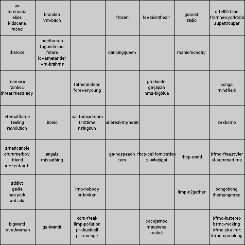
The figure above represents the standard SOM grid of a 7x7 SOM.
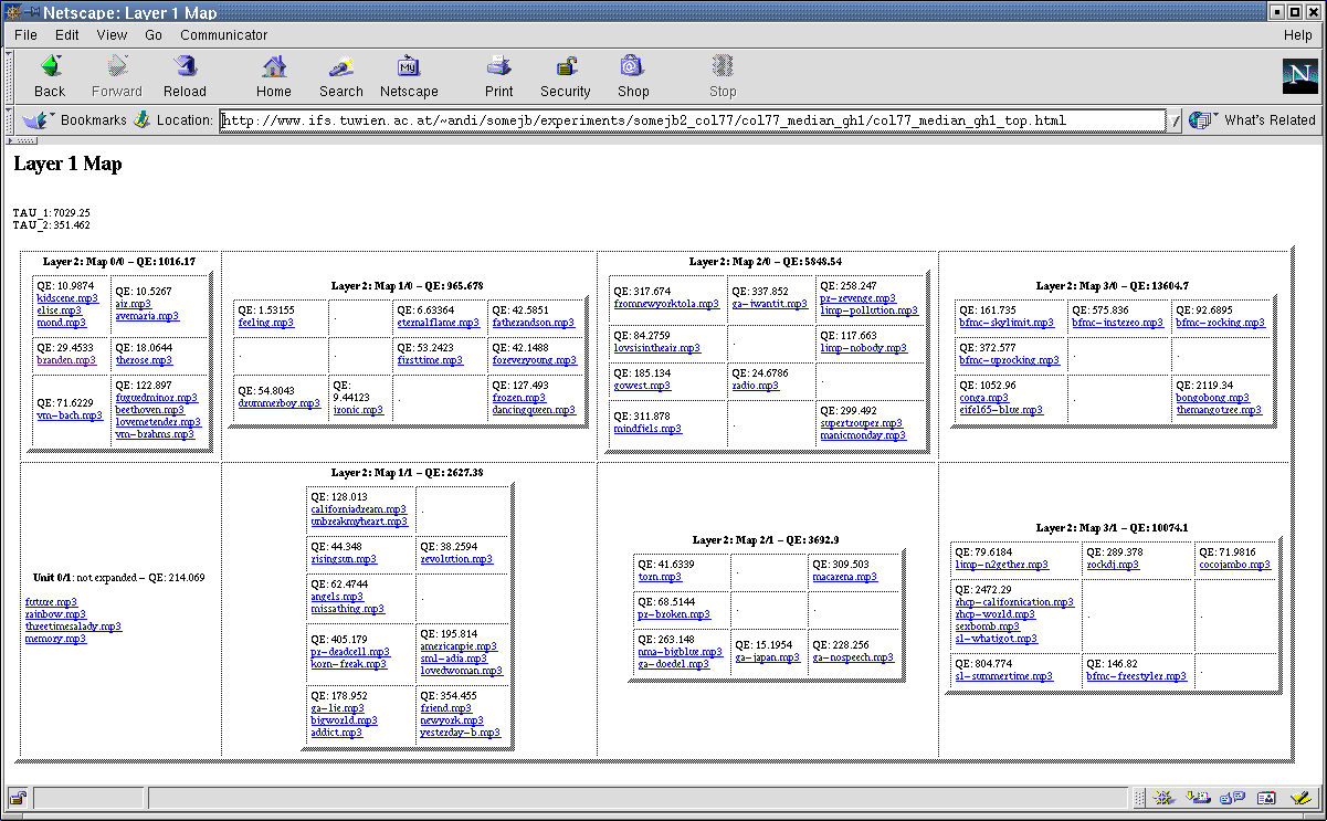
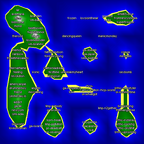
If we apply the SDH visualization, we obtain the cluster representation depicted in the figure below. An interactive map, with the MP3 files linked to is provided right afterwards.
In the map below you will find the same clusters, yet interactive links to the MP3 files allow you to explore the clustering, to listen to the various sound characteristics, and get an impression of how the map organized the pieces of music. In the following step, we will take a closer look at the characteristic features that can be extracted from the mappings.
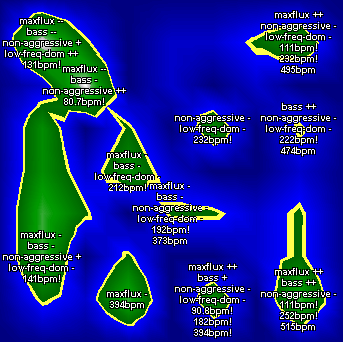
The following image shows how peaks can be labeled to help navigation on the
map. Basically, we can take a look at the values for each of the features separately, resulting in so-called component planes.
Since the single dimensions are not very informative aggregated attributes can be formed from these and can be used to summarize characteristics of the clusters. There are several possibilities to form aggregated attributes, for example, using the sum, mean, or median of all or only a subset of the dimensions. Furthermore, it is possible to compare different subsets to each other. In the following 4 aggregated attributes, which point out some of the possibilities, are presented. If the user understands the MFS it is possible that the user directly creates the aggregated attributes depending on personal preferences.
The used aggregated attributes are Maximum Fluctuation Strength, Bass, Non-Aggressive, and Low Frequencies Dominant. The names have been chosen to indicate what they describe.
All peaks above the sea level (mountains and hills) have been labeled with
descriptions. For example, the islands located at
the upper left corner of the map is labeled maxflux ++, non-aggressive -,
low-freq-dom +, 111bpm!, 232bpm!, 495bpm. These labels indicate disco music.
(Up to the top of the page)
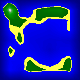
We start with a representation of the low-frequencies dominating attribute, depicted below. The low-freq-dom is high for pieces of music where mostly the lower frequencies are active. There are two groups where this is the case. One is classical music like F³r Elise by Beethoven. The other is music with a strong bass like the songs by Bomfunk MC's.
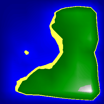
In the figure below, areas on the map are highlighted that have a strong bass beat. On this map the songs, which have the highest bass values, are located in the
lower right corner and are from Bomfunk MC's. There is a strong correlation
between the bass and the maxflux, which we will take a look at in the subsequent image.
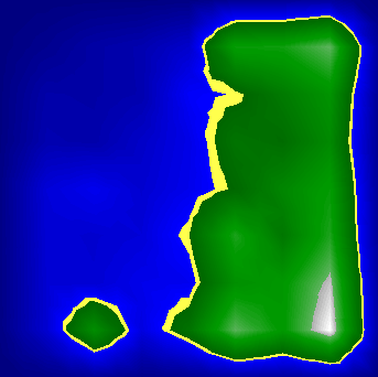
In the figure below we can now take a closer look at which areas on the map have high or low maxflux values. The maximum fluctuation strength is high for pieces of music that have a strong
re-occurring beat. On this map the songs, which have the highest maxflux
values, are located in the lower right corner and are from Bomfunk MC's.
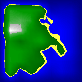
Last, but not least, we will take a look at an attribute entitled non-aggressive. The non-aggressive is high for pieces of music that don't have a strong re-occurring fast beat. On this map a song, which has very high non-aggressive values, is Memory by Barbara Streisand.
(Up to the top of the page)
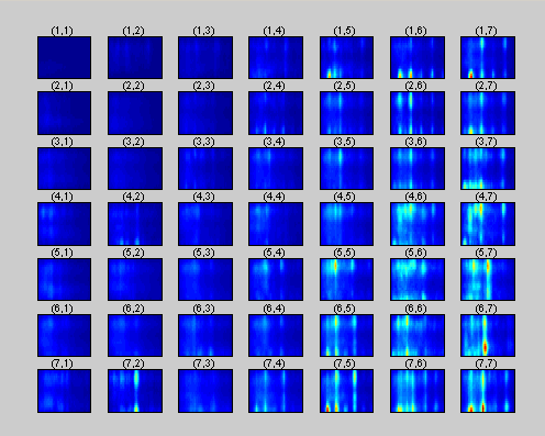
The figure below shows the un-scaled model vectors. They represent the data the same way the SOM algorithm sees them. Each model vector is titled with its coordinates on the 7x7 SOM.
The linear x-axis of each MV represents the modulation frequency in the range
from 0-10Hz. The y-axis represents the critical-band rate scale in the range
from 1-20 Bark.
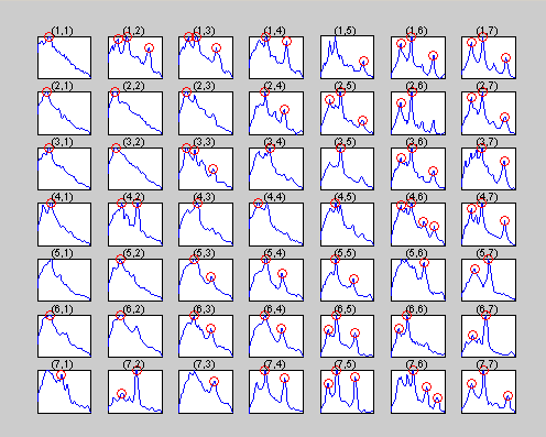
Last, but not least, we provide a rhythmic representation of each model vector.
The images are created by summing up the MFS values over the critical-band
rate scale and normalizing them so that their maximum equals one.
Peeks are subsequently selected using a simple heuristic.
(Up to the top of the page)
4. Islands of Music
We now present the Islands of Music interface to a flat SOM trained with the 77-Collection, and take a look at the various component planes of the resulting SOM.
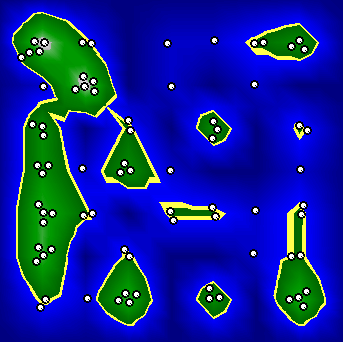
Click on the white bullets to liste to the music files (requires
MP3-plugin)
5. Component Planes
We will now take a look at the various component planes of the map.
Characteristic behavior of music in certain frequency ranges can be mapped onto a specific acoustic impression.
Below we provide figures of the intensity distributions of some of these features across the map.
6. Model Vectors
Of course, we may also take a look at the characteristics of the model vectors, to see which patterns they represent, and thus, for which type of music they are a prototype for.
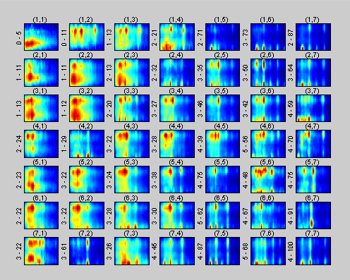
The figure below represents the scale model vectors. The color scale of each model vector is adjusted to best fit the MFS data.
Each model vector is titled with its coordinates on the 7x7 SOM. To the left of
each model vector are values that indicate the range of the MFS values relative
to the whole collection, where 0 is the lowest and 100 the highest value.
The linear x-axis of each model vector represents the modulation frequency in the range
from 0-10Hz. The y-axis represents the critical-band rate scale in the range
from 1-20 Bark.
